“Buying a house is a stressful thing.”
Contrary to the widespread belief that house prices are dependent on the generic factors like number of bedrooms and square area of house, Ames Housing dataset proves that many other factors influence the final price of homes. This dataset contains 79 explanatory variables to describe almost every aspect of the house. Generally house buyers neglect this information. As a result their price estimation is very different from the actual prices.
Below is my first Data Science Project as part of Data Mining Course, a model to predict the prices of residential homes in Ames, Iowa, using advanced regression techniques. This will provide buyers will a rough estimate of what the houses are actually worth. This in turn will help them have better negotiation deals with sellers.
Most of the houses are bought through real estate agents. People rarely buy directly from the seller, since there are a lot of legal terminology involved and people are unaware of them. Hence real estate agents are trusted with the communication between buyers and sellers as well as laying down a legal contract for the transfer. This just creates a middle man and increases the cost of houses. Therefore the houses are overpriced and a buyer should have a better idea of the actual value of these houses.[2] There are various tools, like Zillow and Trulia, available online to assist a person with buying houses. These tools provide a price estimation of various houses and are generally free for use. These tools incorporate many factors to estimate the house prices by providing weights to each factor. For example, Zillow creates Zestimate of houses which is “calculated three times a week based on millions of public and user-submitted data points” [3]. The median error rate for these estimates are quite low. The main problem with these tools is that they are heavy on advertisements and they promote real estate agents. Zillow provides paid premium services for real estate agents and this is their main source of income.[4]
Estimates of actual house prices will help buyers to have better negotiations with the real estate agents, as the list price of the house and much higher than the actual price. Our prediction model will provide the buyers with these estimates.
We used the ‘Ames Housing dataset’ provided by [kaggle](https://www.kaggle.com/) for competition [House Prices: Advanced Regression Techniques](https://www.kaggle.com/c/house-prices-advanced-regression-techniques).
Python Packages
import warnings
import numpy as np
import pandas as pd
%matplotlib inline
%config InlineBackend.figure_format = 'png' #retina
import matplotlib.pyplot as plt
import seaborn as sns
import warnings
warnings.filterwarnings('ignore')
import scipy.stats as stats
from scipy.stats import skew,norm
from scipy.stats.stats import pearsonr
Data Preprocessing
train = pd.read_csv("./train.csv")
test = pd.read_csv("./test.csv")

#Save the 'Id' column
train_ID = train['Id']
test_ID = test['Id']

#Now drop the  'Id' colum since it's unnecessary for  the prediction process.
train.drop("Id", axis = 1, inplace = True)
test.drop("Id", axis = 1, inplace = True)
We performed following statisitical analysis of the data for finding trends in data.
DataFrame Properties
print('Train Data: \n')
print("Number of columns: "+ str(train.shape[1]))
print("Number of rows: "+ str(train.shape[0]))
print('\nTest Data: \n')
print("Number of columns: "+ str(test.shape[1]))
print("Number of rows: "+ str(test.shape[0]))
Train Data:

Number of columns: 80
Number of rows: 1460

Test Data:

Number of columns: 79
Number of rows: 1459
Statistical data summary
train['SalePrice'].describe()
count      1460.000000
mean     180921.195890
std       79442.502883
min       34900.000000
25%      129975.000000
50%      163000.000000
75%      214000.000000
max      755000.000000
Name: SalePrice, dtype: float64
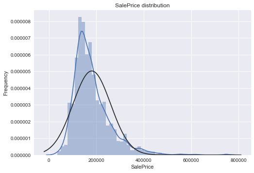
# Kernel Density Plot
sns.distplot(train.SalePrice,fit=norm);
plt.ylabel('Frequency')
plt.title('SalePrice distribution');
# Get the fitted parameters used by the function
(mu, sigma) = norm.fit(train['SalePrice']);
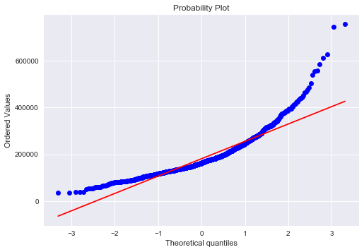
# QQ-plot
fig = plt.figure()
res = stats.probplot(train['SalePrice'], plot=plt)
plt.show()
 ](http://rahulraghatate.github.io/img/Property-Evaluation/output_6_0.png)
 ](http://rahulraghatate.github.io/img/Property-Evaluation/output_6_1.png)
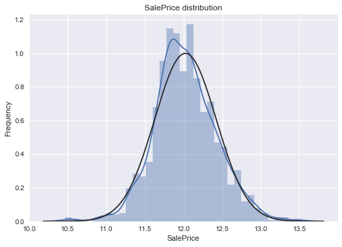
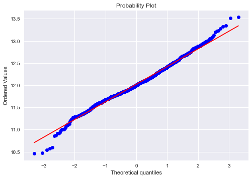
The target variable is right skewed(positive skewness) and show peakedness. As (linear) models fits better on normally distributed data , we require proper transformation.
Transform the skewed numeric features by taking log(feature + 1) - to make features more normal
Relation Exploration for Few Numerical Variables
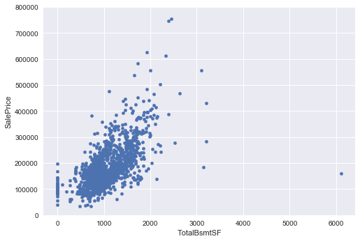
#scatter plot totalbsmtsf/saleprice
var = 'TotalBsmtSF'
data = pd.concat([train['SalePrice'], train[var]], axis=1)
data.plot.scatter(x=var, y='SalePrice', ylim=(0,800000));
 ](http://rahulraghatate.github.io/img/Property-Evaluation/output_9_0.png)
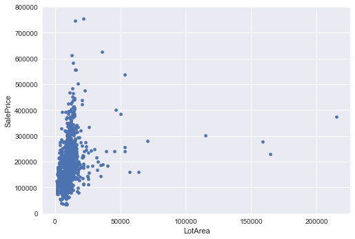
#scatter plot LotArea/saleprice
var = 'LotArea'
data = pd.concat([train['SalePrice'], train[var]], axis=1)
data.plot.scatter(x=var, y='SalePrice', ylim=(0,800000));
 ](http://rahulraghatate.github.io/img/Property-Evaluation/output_10_0.png)
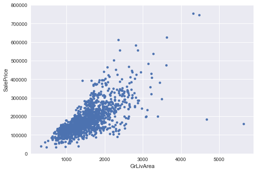
#scatter plot grlivarea/saleprice
var = 'GrLivArea'
data = pd.concat([train['SalePrice'], train[var]], axis=1)
data.plot.scatter(x=var, y='SalePrice', ylim=(0,800000));
 ](http://rahulraghatate.github.io/img/Property-Evaluation/output_11_0.png)
Deleting outliers
train = train.drop(train[(train['GrLivArea']>4000) & (train['SalePrice']<300000)].index)
‘TotalBsmtSF’,’LotArea’ and ‘GrLivArea’ seem to be linearly related with ‘SalePrice’. Both relationships are positive, which means that as one variable increases, the other also increases. In the case of ‘TotalBsmtSF’ and ‘LotArea’ we can see that the slope of the linear relationship are particularly high.
Relation Exploration for categorical features
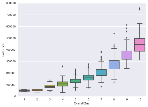
#box plot overallqual/saleprice
var = 'OverallQual'
data = pd.concat([train['SalePrice'], train[var]], axis=1)
f, ax = plt.subplots(figsize=(8, 6))
fig = sns.boxplot(x=var, y="SalePrice", data=data)
fig.axis(ymin=0, ymax=800000);
 ](http://rahulraghatate.github.io/img/Property-Evaluation/output_15_0.png)
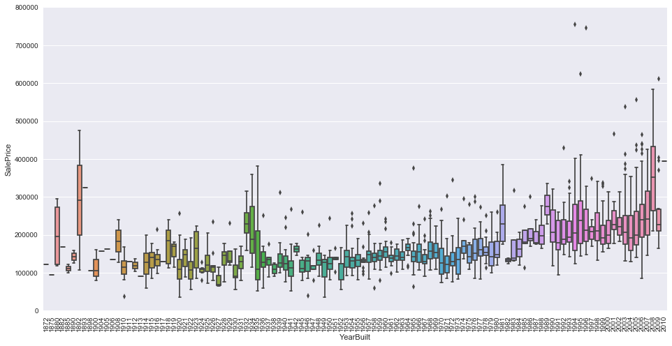
var = 'YearBuilt'
data = pd.concat([train['SalePrice'], train[var]], axis=1)
f, ax = plt.subplots(figsize=(16, 8))
fig = sns.boxplot(x=var, y="SalePrice", data=data)
fig.axis(ymin=0, ymax=800000);
plt.xticks(rotation=90);
 ](http://rahulraghatate.github.io/img/Property-Evaluation/output_16_0.png)
Note: we don’t know if ‘SalePrice’ is in constant prices. Constant prices try to remove the effect of inflation. If ‘SalePrice’ is not in constant prices, it should be, so than prices are comparable over the years.
OverallQual’ and ‘YearBuilt’ also seem to be related with ‘SalePrice’. The relationship seems to be stronger in the case of ‘OverallQual’, where the box plot shows how sales prices increase with the overall quality.
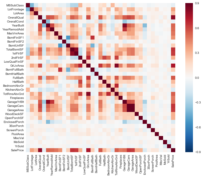
correlation matrix for all features
corrmat = train.corr()
f, ax = plt.subplots(figsize=(12, 9))
sns.heatmap(corrmat, vmax=.9, square=True);
 ](http://rahulraghatate.github.io/img/Property-Evaluation/output_19_0.png)
#skewness and kurtosis
print("Skewness: %f" % train['SalePrice'].skew())
print("Kurtosis: %f" % train['SalePrice'].kurt())
Skewness: 1.881296
Kurtosis: 6.523067
log transforming the target and Kernel Density plot for Sale Price values
train["SalePrice"] = np.log1p(train["SalePrice"])
# Kernel Density Plot
sns.distplot(train.SalePrice,fit=norm);
plt.ylabel('Frequency')
plt.title('SalePrice distribution');
# Get the fitted parameters used by the function
(mu, sigma) = norm.fit(train['SalePrice']);
# QQ-plot
fig = plt.figure()
res = stats.probplot(train['SalePrice'], plot=plt)
plt.show()
 ](http://rahulraghatate.github.io/img/Property-Evaluation/output_21_0.png)
 ](http://rahulraghatate.github.io/img/Property-Evaluation/output_21_1.png)
_Sample training dataframe__
train.head()
| MSSubClass | MSZoning | LotFrontage | LotArea | Street | Alley | LotShape | LandContour | Utilities | LotConfig | ... | PoolArea | PoolQC | Fence | MiscFeature | MiscVal | MoSold | YrSold | SaleType | SaleCondition | SalePrice | |
|---|---|---|---|---|---|---|---|---|---|---|---|---|---|---|---|---|---|---|---|---|---|
| 0 | 60 | RL | 65.0 | 8450 | Pave | NaN | Reg | Lvl | AllPub | Inside | ... | 0 | NaN | NaN | NaN | 0 | 2 | 2008 | WD | Normal | 12.247699 |
| 1 | 20 | RL | 80.0 | 9600 | Pave | NaN | Reg | Lvl | AllPub | FR2 | ... | 0 | NaN | NaN | NaN | 0 | 5 | 2007 | WD | Normal | 12.109016 |
| 2 | 60 | RL | 68.0 | 11250 | Pave | NaN | IR1 | Lvl | AllPub | Inside | ... | 0 | NaN | NaN | NaN | 0 | 9 | 2008 | WD | Normal | 12.317171 |
| 3 | 70 | RL | 60.0 | 9550 | Pave | NaN | IR1 | Lvl | AllPub | Corner | ... | 0 | NaN | NaN | NaN | 0 | 2 | 2006 | WD | Abnorml | 11.849405 |
| 4 | 60 | RL | 84.0 | 14260 | Pave | NaN | IR1 | Lvl | AllPub | FR2 | ... | 0 | NaN | NaN | NaN | 0 | 12 | 2008 | WD | Normal | 12.429220 |
5 rows × 80 columns
Exploring Missing value ratio
all_data = pd.concat((train.loc[:,'MSSubClass':'SaleCondition'],
                      test.loc[:,'MSSubClass':'SaleCondition']))

print("all_data size is : {}".format(all_data.shape))
all_data_na = (all_data.isnull().sum() / len(all_data)) * 100
all_data_na = all_data_na.drop(all_data_na[all_data_na == 0].index).sort_values(ascending=False)[:30]
missing_data = pd.DataFrame({'Missing Ratio' :all_data_na})
missing_data.head(20)
all_data size is : (2917, 79)
| Missing Ratio | |
|---|---|
| PoolQC | 99.691464 |
| MiscFeature | 96.400411 |
| Alley | 93.212204 |
| Fence | 80.425094 |
| FireplaceQu | 48.680151 |
| LotFrontage | 16.660953 |
| GarageFinish | 5.450806 |
| GarageYrBlt | 5.450806 |
| GarageQual | 5.450806 |
| GarageCond | 5.450806 |
| GarageType | 5.382242 |
| BsmtExposure | 2.811107 |
| BsmtCond | 2.811107 |
| BsmtQual | 2.776826 |
| BsmtFinType2 | 2.742544 |
| BsmtFinType1 | 2.708262 |
| MasVnrType | 0.822763 |
| MasVnrArea | 0.788481 |
| MSZoning | 0.137127 |
| BsmtFullBath | 0.068564 |
Imputing missing values
Based on feature description provided, following features if has NA means it’s absent(“None”).
for col in ('PoolQC','MiscFeature','GarageType','Alley','Fence','FireplaceQu','GarageFinish', 'GarageQual', 'GarageCond','MasVnrType','MSSubClass'):
    all_data[col] = all_data[col].fillna('None')

# Replacing missing data with 0 (Since No garage = no cars in such garage).

for col in ('GarageYrBlt', 'GarageArea', 'GarageCars'):
    all_data[col] = all_data[col].fillna(0)
# missing values are likely zero for having no basement

for col in ('BsmtFinSF1', 'BsmtFinSF2', 'BsmtUnfSF','TotalBsmtSF', 'BsmtFullBath', 'BsmtHalfBath'):
    all_data[col] = all_data[col].fillna(0)
#
all_data["MasVnrArea"] = all_data["MasVnrArea"].fillna(0)
# For below categorical basement-related features, NaN means that there is no basement.

for col in ('BsmtQual', 'BsmtCond', 'BsmtExposure', 'BsmtFinType1', 'BsmtFinType2'):
    all_data[col] = all_data[col].fillna('None')

# Group by neighborhood and fill in missing value by the median LotFrontage of all the neighborhood

all_data["LotFrontage"] = all_data.groupby("Neighborhood")["LotFrontage"].transform(
    lambda x: x.fillna(x.median()))

# Setting mode value for missing entries

# MSZoning classification : 'RL' is common
all_data['MSZoning'] = all_data['MSZoning'].fillna(all_data['MSZoning'].mode()[0])

# Functional : NA = typical
all_data["Functional"] = all_data["Functional"].fillna("Typ")

# Electrical
all_data['Electrical'] = all_data['Electrical'].fillna(all_data['Electrical'].mode()[0])

# KitchenQual
all_data['KitchenQual'] = all_data['KitchenQual'].fillna(all_data['KitchenQual'].mode()[0])

# Exterior1st and Exterior2nd
all_data['Exterior1st'] = all_data['Exterior1st'].fillna(all_data['Exterior1st'].mode()[0])
all_data['Exterior2nd'] = all_data['Exterior2nd'].fillna(all_data['Exterior2nd'].mode()[0])

#SaleType
all_data['SaleType'] = all_data['SaleType'].fillna(all_data['SaleType'].mode()[0])
#  Dropping as same value 'AllPub' for all records except 2 NA and 1 'NoSeWa'
all_data = all_data.drop(['Utilities'], axis=1)
# Transformation required for numerical features to categorical

all_data['MSSubClass'] = all_data['MSSubClass'].apply(str)
all_data['OverallCond'] = all_data['OverallCond'].astype(str)
all_data['YrSold'] = all_data['YrSold'].astype(str)
all_data['MoSold'] = all_data['MoSold'].astype(str)
Label Encoding some categorical variables for information in their ordering set
from sklearn.preprocessing import LabelEncoder
cols = ('FireplaceQu', 'BsmtQual', 'BsmtCond', 'GarageQual', 'GarageCond',
        'ExterQual', 'ExterCond','HeatingQC', 'PoolQC', 'KitchenQual', 'BsmtFinType1',
        'BsmtFinType2', 'Functional', 'Fence', 'BsmtExposure', 'GarageFinish', 'LandSlope',
        'LotShape', 'PavedDrive', 'Street', 'Alley', 'CentralAir', 'MSSubClass', 'OverallCond',
        'YrSold', 'MoSold')
# process columns, apply LabelEncoder to categorical features
for c in cols:
    lbl = LabelEncoder()
    lbl.fit(list(all_data[c].values))
    all_data[c] = lbl.transform(list(all_data[c].values))

# shape
print('Shape all_data: {}'.format(all_data.shape))
Shape all_data: (2917, 78)
# Adding Total surface area as 'TotalSF'= basement+firstflr+secondflr

all_data['TotalSF'] = all_data['TotalBsmtSF'] + all_data['1stFlrSF'] + all_data['2ndFlrSF']
log transform skewed numeric features
numeric_feats = all_data.dtypes[all_data.dtypes != "object"].index
skewed_feats = all_data[numeric_feats].apply(lambda x: skew(x.dropna())).sort_values(ascending=False) #compute skewness
print("\nSkew in numerical features: \n")
skewness = pd.DataFrame({'Skew' :skewed_feats})
skewness.head(5)
Skew in numerical features:
| Skew | |
|---|---|
| MiscVal | 21.939672 |
| PoolArea | 17.688664 |
| LotArea | 13.109495 |
| LowQualFinSF | 12.084539 |
| 3SsnPorch | 11.372080 |
Box Cox Transformation of (highly) skewed features
skewness = skewness[abs(skewness) > 0.75]
print("There are {} skewed numerical features to Box Cox transform".format(skewness.shape[0]))

from scipy.special import boxcox1p
skewed_features = skewness.index
lam = 0.15
for feat in skewed_features:
    all_data[feat] = boxcox1p(all_data[feat], lam)
There are 59 skewed numerical features to Box Cox transform
Dummy Variables for categorical features
all_data = pd.get_dummies(all_data)
print(all_data.shape)
(2917, 220)
ntrain = train.shape[0]
ntest = test.shape[0]
y_train= train.SalePrice.values
train = pd.DataFrame(all_data[:ntrain])
test = pd.DataFrame(all_data[ntrain:])
Regression Modeling
Importing Sklearn Packages for Modeling
from sklearn.linear_model import ElasticNet, Lasso,  BayesianRidge, LassoLarsIC
from sklearn.ensemble import RandomForestRegressor,  GradientBoostingRegressor
from sklearn.kernel_ridge import KernelRidge
from sklearn.pipeline import make_pipeline
from sklearn.preprocessing import RobustScaler
from sklearn.base import BaseEstimator, TransformerMixin, RegressorMixin, clone
from sklearn.model_selection import KFold, cross_val_score, train_test_split
from sklearn.metrics import mean_squared_error
import xgboost as xgb
import lightgbm as lgb
For Cross-validation purpose we can use cross_val_score function of Sklearn. However this function has not a shuffle attribut, we add then one line of code on Alexandru function, in order to shuffle the dataset prior to cross-validation
#Validation function
n_folds = 5

def rmsle_cv(model):
    kf = KFold(n_folds, shuffle=True, random_state=42).get_n_splits(train.values)
    rmse= np.sqrt(-cross_val_score(model, train.values, y_train, scoring="neg_mean_squared_error", cv = kf))
    return(rmse)
Implementation of following Regression Models
1. Lasso Regression
2. Kernel Ridge Regression
3. Elastic Net Regression
4. Gradient Boosting Regression
5. XGBoost
6. Light GBM
Model Parameters Setting
#1
lasso = make_pipeline(RobustScaler(), Lasso(alpha =0.0005, random_state=1))
#2
KRR = KernelRidge(alpha=0.6, kernel='polynomial', degree=2, coef0=2.5)
#3
ENet = make_pipeline(RobustScaler(), ElasticNet(alpha=0.0005, l1_ratio=.9, random_state=3))
#4
GBoost = GradientBoostingRegressor(n_estimators=3000, learning_rate=0.05,
                                   max_depth=4, max_features='sqrt',
                                   min_samples_leaf=15, min_samples_split=10,
                                   loss='huber', random_state =5)
#5
model_xgb = xgb.XGBRegressor(colsample_bytree=0.4603, gamma=0.0468,
                             learning_rate=0.05, max_depth=3,
                             min_child_weight=1.7817, n_estimators=2200,
                             reg_alpha=0.4640, reg_lambda=0.8571,
                             subsample=0.5213, silent=1,seed=7, nthread = -1)
#6
model_lgb = lgb.LGBMRegressor(objective='regression',num_leaves=5,
                              learning_rate=0.05, n_estimators=720,
                              max_bin = 55, bagging_fraction = 0.8,
                              bagging_freq = 5, feature_fraction = 0.2319,
                              feature_fraction_seed=9, bagging_seed=9,
                              min_data_in_leaf =6, min_sum_hessian_in_leaf = 11)
**Scores for Base Models
score = rmsle_cv(lasso)
print("\nLasso score: {:.4f} ({:.4f})\n".format(score.mean(), score.std()))

score = rmsle_cv(KRR)
print("Kernel Ridge score: {:.4f} ({:.4f})\n".format(score.mean(), score.std()))

score = rmsle_cv(ENet)
print("ElasticNet score: {:.4f} ({:.4f})\n".format(score.mean(), score.std()))

score = rmsle_cv(GBoost)
print("Gradient Boosting score: {:.4f} ({:.4f})\n".format(score.mean(), score.std()))

score = rmsle_cv(model_xgb)
print("Xgboost score: {:.4f} ({:.4f})\n".format(score.mean(), score.std()))

score = rmsle_cv(model_lgb)
print("LGBM score: {:.4f} ({:.4f})\n" .format(score.mean(), score.std()))
Lasso score: 0.1115 (0.0074)

Kernel Ridge score: 0.1153 (0.0075)

ElasticNet score: 0.1116 (0.0074)

Gradient Boosting score: 0.1167 (0.0084)

Xgboost score: 0.1165 (0.0058)

LGBM score: 0.1156 (0.0069)
Stacking Models
Approach: Averaging Base Models
#Average Based models class

class AveragingModels(BaseEstimator, RegressorMixin, TransformerMixin):
    def __init__(self, models):
        self.models = models

    # we define clones of the original models to fit the data in
    def fit(self, X, y):
        self.models_ = [clone(x) for x in self.models]

        # Train cloned base models
        for model in self.models_:
            model.fit(X, y)

        return self

    #Now we do the predictions for cloned models and average them
    def predict(self, X):
        predictions = np.column_stack([
            model.predict(X) for model in self.models_
        ])
        return np.mean(predictions, axis=1)


# Averaged base models score

averaged_models = AveragingModels(models = (ENet, GBoost, KRR, lasso))

score = rmsle_cv(averaged_models)
print(" Averaged base models score: {:.4f} ({:.4f})\n".format(score.mean(), score.std()))
Averaged base models score: 0.1087 (0.0077)
Defining rmsle evaluation function
def rmsle(y, y_pred):
    return np.sqrt(mean_squared_error(y, y_pred))
Training and Prediction for Stacked Model
#StackedRegressor:

averaged_models.fit(train.values, y_train)
stacked_train_pred = averaged_models.predict(train.values)
stacked_pred = np.expm1(averaged_models.predict(test.values))
print(rmsle(y_train, stacked_train_pred))
0.0794023865241
XGBoost_Model and LightGBM(Gradient_Boosted_Model)
model_xgb.fit(train, y_train)
xgb_train_pred = model_xgb.predict(train)
xgb_pred = np.expm1(model_xgb.predict(test))
print(rmsle(y_train, xgb_train_pred))

model_lgb.fit(train, y_train)
lgb_train_pred = model_lgb.predict(train)
lgb_pred = np.expm1(model_lgb.predict(test.values))
print(rmsle(y_train, lgb_train_pred))
0.0782418795595
0.0724680051983
'''RMSE on the entire Train data when averaging'''

print('RMSLE score on train data:')
print(rmsle(y_train,stacked_train_pred*0.70 +
               xgb_train_pred*0.15 + lgb_train_pred*0.15 ))
RMSLE score on train data:
0.0759625096638
Ensembled Final Predictions
ensemble = stacked_pred*0.70 + xgb_pred*0.15 + lgb_pred*0.15
sub = pd.DataFrame()
sub['Id'] = test_ID
sub['SalePrice'] = ensemble
sub.to_csv('submission.csv',index=False)