This report provides primary analysis of Pew-Research-Center-National-Identity-Report-Data
Load Required Libraries
library(ggplot2)
library(grid)
library(GGally)
Reading Data into R
birthplace<-read.csv('birthplace.csv',header = FALSE,fileEncoding = 'UTF-8-BOM')
language<-read.csv('language.csv',header = FALSE,fileEncoding = 'UTF-8-BOM')
religion<-read.csv('religion.csv',header = FALSE,fileEncoding = 'UTF-8-BOM')
customs<-read.csv('customs.csv',header = FALSE,fileEncoding = 'UTF-8-BOM')
Standardizing scores for all four Questions
birthplace["score"]<-(4*birthplace[2]+3*birthplace[3]+2*birthplace[4]
                      +birthplace[5])/(birthplace[2]+birthplace[3]+birthplace[4]+birthplace[5])
language["score"]<-(4*language[2]+3*language[3]+2*language[4]
                    +language[5])/(language[2]+language[3]+language[4]+language[5])
religion["score"]<-(4*religion[2]+3*religion[3]+2*religion[4]
                    +religion[5])/(religion[2]+religion[3]+religion[4]+religion[5])
customs["score"]<-(4*customs[2]+3*customs[3]+2*customs[4]
                   +customs[5])/(customs[2]+customs[3]+customs[4]+customs[5])
Replace NAN value for Japan
religion<- replace(religion,is.na(religion),0)
Calculate Z score (Standardization)
birthplace$score<-(birthplace$score-mean(birthplace$score))/sd(birthplace$score)
language$score<-(language$score-mean(language$score))/sd(language$score)
religion$score<-(religion$score-mean(religion[1:13,"score"]))/sd(religion[1:13,"score"])
customs$score<-(customs$score-mean(customs$score))/sd(customs$score)
religion[14,8]<-0
countries<-birthplace[1]
Data_Frame
data<-cbind(countries,birthplace$score,language$score,religion$score,customs$score)
colnames(data)<-c("country","birth_score","lang_score","rel_score","cust_score")
Univariate Analysis
#total score for each country (adding up the standardized scores for all four questions)
uni_data<-cbind(countries,round(birthplace$score+language$score+religion$score+customs$score,2))

colnames(uni_data)<-c("country","stan_score")

uni_data <- uni_data[order(uni_data$stan_score), ] # sort

# convert to factor to retain sorted order in plot.
uni_data$`country` <- factor(uni_data$`country`, levels = uni_data$`country`)

# Resultant graph with the country ordered by their total score.
ggplot(uni_data, aes(x=`country`, y=stan_score, label=stan_score)) +
  geom_point(stat='identity', fill="black", size=6) +
  geom_text(color="white", size=2) +
  labs(title="Dot plot for standardized_total_score data for countries",
       subtitle="22 country")+coord_flip()

Bivariate Analysis
bi_data<-data[c(2:5)]

#scatterplot matrix for four questions data
ggpairs(data,columns=c(2:5))
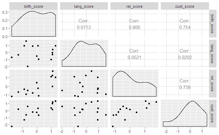
From the above scatterplot matrix its evident that,
- birthplace and customs (corr=0.754), customs and religion (corr=0.739), religion and birthplace (corr=0.806) are strongly related.
- Correlation for pairs (language,customs), (language,religion), (birthplace,language) shows that language is very weakly related to birthplace,religion,customs.
Trivariate Analysis
From language its evident that birthplace-religion-customs are strongly related variables and language doesn’t seem to be related to any other.It seems, birthplace is highly correlated with religion and customs. So, we will make chopped language and add color:
#Taking two sets of values of language (above and below mean) for two colors
lang.cat<-cut_number(data$lang_score,n=2,labels=c("BM","AM"))
#Scatterplot Matrix of
ggpairs(data.frame(data[, 2:5], lang.cat), aes(color = lang.cat),title = "Scatterplot Matrix")
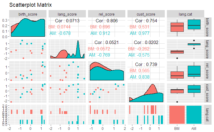
We see that, there is no clear pattern(relation) between any other variables for higher(above mean) and lower values(below mean) of lang_score.
Even if considered,for higher values of lang_score, birthplace and religion are highly correlated(0.912) but no clear pattern to detect it from graph. Its indicative from scatterplot between birth_score and cust_score that for higher values(above mean) of lang_score they are showing linear relation(green dots). The countries with higher lang_scores are tending to show higher religion score that birth_score.Due to trivariate analysis only its evident, else in bivariate plot, it would be misleading as all the datapoints would be of same color.